Table of Contents
Introduction
The ability to access high frequency 100 Hz data is not currently possible with the catapultR package. However, it is possible to access a 100 Hz CSV for each athlete by date in your local OpenField files. Bear in mind that these files are big and will consume a lot of space on your hard drive.
Generate 100 Hz CSV with OpenField Console
After making sure that the required HighFreq module has been enabled on your OpenField console, follow the steps:
- Open OF (Restart OF if already open)
- Click on ‘Data Transfer’
- Hit ‘Stop Transfer’
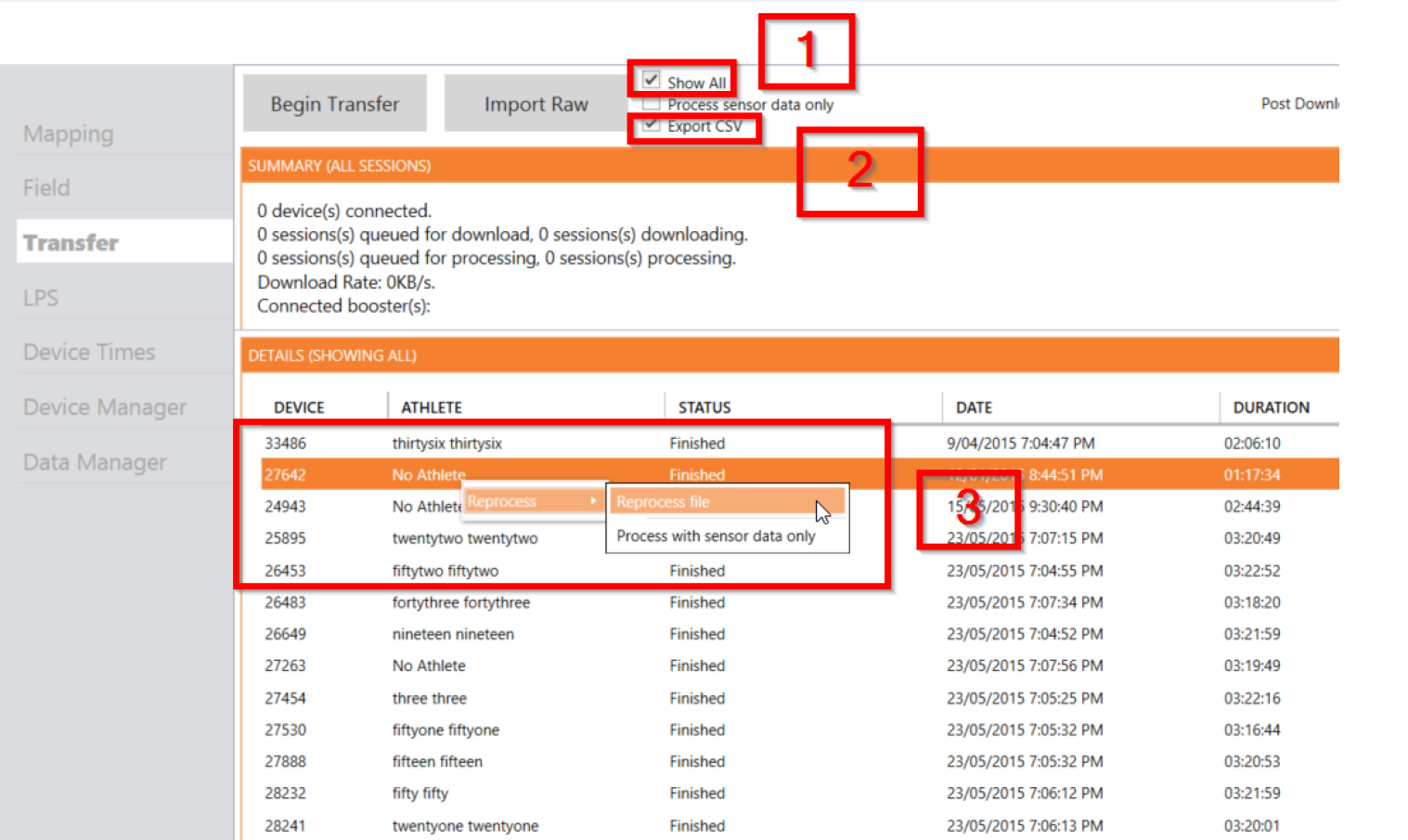
- Select ‘Export CSV’ and ‘Show All’ (setp 1 and 2 in the below screenshot)
- Right Click to reprocess file(s) to get 100hz data from previously downloaded (step 3). You can sort by date, unit, or athlete name. To select multiple files hold down the control key to choose 1 at a time or hold shift to select sections.
- Files will be located in:
Documents/Catapult Sports/OpenField/Analytics/CSV/[Year]/[Month]/[Day]
Reading in a 100 Hz CSV
The function read_CATCSV() can then be used to read in this file when the filepath is specified as an argument. It will return a list the following elements:
- data: the actual 100 Hz data with a column for each variable
- RefTime: the date and time of the start of the file
- DatesOnly: the date of the start of the file
- TimeOnly: the UTC time of the start of the file in hh:mm:ss format
- DeviceID: the id of the Catapult device
- DeviceFamily: the family of the device (e.g. S6)
- OFVersion: the version of OpenField used when device was synced
- FirmwareVersion: the version of the firmware on the device
- CentisecTime: The unix time in centiseconds at the start of the file
library(catapultR)

high_freq <- read_CATcsv(filedatapath = "data/10170_1574708954_1309.csv")
str(high_freq)
List of 9
 $ data           : spec_tbl_df [32,117 x 30] (S3: spec_tbl_df/tbl_df/tbl/data.frame)
  ..$ Acceleration.forward   : num [1:32117] -1.002 -0.998 -0.994 -0.99 -0.973 ...
  ..$ Acceleration.side      : num [1:32117] 0.000484 0.001936 0.001936 0.003388 0.010648 ...
  ..$ Acceleration.up        : num [1:32117] 0.173 0.182 0.184 0.188 0.181 ...
  ..$ Rotation.roll          : num [1:32117] 1.83 1.891 1.342 0.671 0.061 ...
  ..$ Rotation.pitch         : num [1:32117] -0.366 -0.183 -0.488 0.061 0.061 -0.488 -0.854 -0.854 -0.671 -0.061 ...
  ..$ Rotation.yaw           : num [1:32117] 0.366 0.732 1.586 0.976 1.83 ...
  ..$ RawPlayerLoad          : num [1:32117] 0.5376 0.2515 0.1157 0.0527 0.0161 ...
  ..$ SmoothedPlayerLoad     : num [1:32117] 0.0831 0.0834 0.0836 0.0836 0.0835 ...
  ..$ RawPlayerLoad2D        : num [1:32117] 0.5303 0.2471 0.1138 0.0518 0.0156 ...
  ..$ RawPlayerLoad1DFwd     : num [1:32117] 0.5303 0.2471 0.1138 0.0518 0.0156 ...
  ..$ RawPlayerLoad1DSide    : num [1:32117] 0 0.000488 0 0.000488 0.003906 ...
  ..$ RawPlayerLoad1DUp      : num [1:32117] 0.09131 0.04785 0.02344 0.01221 0.00195 ...
  ..$ imuAcceleration.forward: num [1:32117] -0.998 -0.99 -0.982 -0.973 -0.952 ...
  ..$ imuAcceleration.side   : num [1:32117] 0.000426 0.001801 0.001736 0.003135 0.01034 ...
  ..$ imuAcceleration.up     : num [1:32117] -0.808 -0.78 -0.76 -0.738 -0.729 ...
  ..$ imuOrientation.forward : num [1:32117] 0.0191 0.0381 0.0569 0.0755 0.0939 ...
  ..$ imuOrientation.side    : num [1:32117] 0.000316 0.00067 0.000942 0.001125 0.001359 ...
  ..$ imuOrientation.up      : num [1:32117] 1 0.999 0.998 0.997 0.996 ...
  ..$ Facing                 : num [1:32117] 180 180 180 180 180 180 180 180 180 180 ...
  ..$ Latitude               : num [1:32117] NA NA NA NA NA NA NA NA NA NA ...
  ..$ Longitude              : num [1:32117] NA NA NA NA NA NA NA NA NA NA ...
  ..$ Odometer               : num [1:32117] NA NA NA NA NA NA NA NA NA NA ...
  ..$ RawVelocity            : num [1:32117] NA NA NA NA NA NA NA NA NA NA ...
  ..$ SmoothedVelocity       : num [1:32117] NA NA NA NA NA NA NA NA NA NA ...
  ..$ GNSS.LPS.Acceleration  : num [1:32117] NA NA NA NA NA NA NA NA NA NA ...
  ..$ MetabolicPower         : num [1:32117] NA NA NA NA NA NA NA NA NA NA ...
  ..$ GNSS.Fix               : num [1:32117] NA NA NA NA NA NA NA NA NA NA ...
  ..$ GNSS.Strength          : num [1:32117] NA NA NA NA NA NA NA NA NA NA ...
  ..$ GNSS.HDOP              : num [1:32117] NA NA NA NA NA NA NA NA NA NA ...
  ..$ HeartRate              : num [1:32117] 0 0 0 0 0 0 0 0 0 0 ...
  ..- attr(*, "spec")=
  .. .. cols(
  .. ..   Acceleration.forward = col_double(),
  .. ..   Acceleration.side = col_double(),
  .. ..   Acceleration.up = col_double(),
  .. ..   Rotation.roll = col_double(),
  .. ..   Rotation.pitch = col_double(),
  .. ..   Rotation.yaw = col_double(),
  .. ..   RawPlayerLoad = col_double(),
  .. ..   SmoothedPlayerLoad = col_double(),
  .. ..   RawPlayerLoad2D = col_double(),
  .. ..   RawPlayerLoad1DFwd = col_double(),
  .. ..   RawPlayerLoad1DSide = col_double(),
  .. ..   RawPlayerLoad1DUp = col_double(),
  .. ..   imuAcceleration.forward = col_double(),
  .. ..   imuAcceleration.side = col_double(),
  .. ..   imuAcceleration.up = col_double(),
  .. ..   imuOrientation.forward = col_double(),
  .. ..   imuOrientation.side = col_double(),
  .. ..   imuOrientation.up = col_double(),
  .. ..   Facing = col_double(),
  .. ..   Latitude = col_double(),
  .. ..   Longitude = col_double(),
  .. ..   Odometer = col_double(),
  .. ..   RawVelocity = col_double(),
  .. ..   SmoothedVelocity = col_double(),
  .. ..   GNSS.LPS.Acceleration = col_double(),
  .. ..   MetabolicPower = col_double(),
  .. ..   GNSS.Fix = col_double(),
  .. ..   GNSS.Strength = col_double(),
  .. ..   GNSS.HDOP = col_double(),
  .. ..   HeartRate = col_double()
  .. .. )
  ..- attr(*, "problems")=<externalptr>
 $ RefTime        : chr "Reference time: 11/25/19 19:09:14 UTC"
 $ DatesOnly      : Date[1:1], format: "2019-11-25"
 $ TimeOnly       : chr "19:09:14"
 $ DeviceID       : chr "10170"
 $ DeviceFamily   : chr "S6"
 $ OFVersion      : chr "2.1.0.999"
 $ FirmwareVersion: chr "6.06"
 $ CentisecTime   : num 1.57e+11
To access the data only, you can use dollar sign notation. The following code accesses the data in the list and plots it. There are several peaks in Raw PlayerLoad because the data corresponds to a baseball player who is throwing a ball every few seconds.
data_only <- high_freq$data

plot(data_only$RawPlayerLoad,
     type = "l", col = "blue",
     main = "Raw PlayerLoad",
     xlab = "Centiseconds", ylab = "Raw PlayerLoad")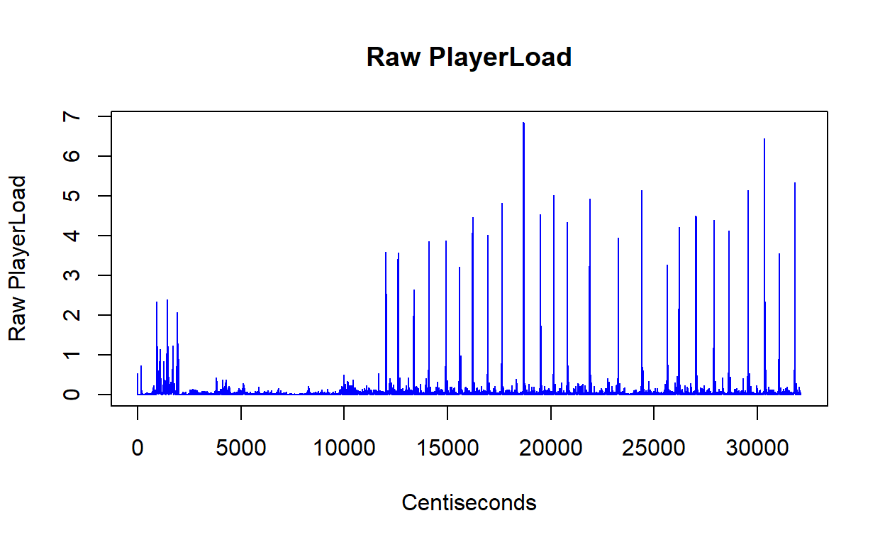
Definitions of the 100 Hz parameters
Contact: Analytics@catapultsports.com (email) | #ask_catapultR (Slack)