Table of Contents
Introduction
Catapult devices monitor athletes continuously throughout training sessions and in games. Measurements of acceleration and rotation are recorded at a rate of 100 Hz (100 times per second). Sometimes this high frequency data is useful, but often a sport scientist will be more interested in summaries of this data over an extended period of time. Catapult users refer to training sessions or games as activities and smaller segments within them as periods. Accessing aggregated summary statistics by activity and period is easily accomplished with the catapultR package.
Validate User Credentials
If enabled on your account, you can also generate an API token string in OpenField Cloud. If you would like this feature enabled on your OpenField account, please speak with your Catapult Sports Customer Success representative.
I will use a Women’s College Soccer demo account for this example, but note that the token string has been generated randomly for presentation purposes only. Typical token strings created in OpenField Cloud will be much longer.
All data presented has been anonymized, removing and changing identifiable characteristics that can be traced back to a team or athlete.
# first, load a few packages
library(catapultR)
library(tidyverse)
library(lubridate)

token <- ofCloudCreateToken(sToken = "STe67MbNGfkO5XH8jaZDyoQvnz4VBYiL0Clg2RcW",  sRegion = "America")
Extracting Aggregated Data
Checking Available Parameters
To see what statistics are available, use the ofCloudGetParameters() function. Find the parameters you want and record the corresponding value from the slug column of the dataframe. A “slug” is a human-readable, unique identifier similar to an id. These slug values will be used as arguments in the next step.
parameters <- ofCloudGetParameters(token)
glimpse(parameters)
Rows: 1,555
Columns: 6
$ id                <chr> "00025054-617c-45f1-ae03-a768ebfcd893", "0~
$ parameter_type_id <chr> "417654ed-209f-4c6f-a028-62c10f873d18", "6~
$ name              <chr> "IMA Accel Medium", "Velocity Band 2 Avera~
$ original_name     <chr> "IMA Accel Medium", "Velocity Band 2 Avera~
$ slug              <chr> "ima_band2_accel_count", "velocity_band2_a~
$ calculation       <chr> "", "", "", "", "", "", "", "", "", "", ""~
Identifying Activities
You may also need to isolate a specific activity of interest. To see the available activities associated with the account, use the ofCloudGetActivities() function. You should then record the activity ID (column id) corresponding to the activity of interest from the resulting dataframe.
activities <- ofCloudGetActivities(token)
glimpse(activities)
Rows: 399
Columns: 19
$ id             <chr> "pkjv7c2u-pf7x-si7l-jldg-axb2lf7vw9c8", "pdvz~
$ name           <chr> "Walkthrough", "Rehab", "Practice", "Practice~
$ start_time     <dbl> 1544530773, 1544375188, 1544276386, 154419436~
$ end_time       <dbl> 1544539319, 1544390043, 1544290470, 154419788~
$ modified_at    <chr> "2020-01-03 21:51:56", "2019-12-13 15:34:24",~
$ game_id        <chr> "pkjv7c2u-pf7x-si7l-jldg-axb2lf7vw9c8", "pdvz~
$ owner_id       <chr> "5311cfa9-c6ee-46da-890a-dfabe8203db4", "5311~
$ owner          <df[,10]> <data.frame[23 x 10]>
$ periods        <list> [<data.frame[5 x 4]>], [<data.frame[1 x 4~
$ tags           <list> <"Practice", "Travel >500 miles", "GPS">, <"~
$ tag_list       <list> [<data.frame[3 x 5]>], [<data.frame[3 x 5]>]~
$ athlete_count  <int> 14, 14, 14, 2, 10, 14, 14, 11, 13, 13, 13, 1~
$ period_count   <int> 5, 1, 1, 1, 2, 8, 5, 5, 4, 3, 6, 6, 2, 8, 2, ~
$ venue_name     <chr> "Training Pitch 3", "Training Pitch 1", "Trai~
$ venue_width    <int> 76, 76, 76, 76, 76, 76, 76, 76, 76, 76, 76, 7~
$ venue_length   <int> 112, 112, 112, 112, 112, 112, 112, 112, 112, ~
$ venue_rotation <int> -89, -89, -89, -89, -89, -89, -89, -89, -89, ~
$ venue_lat      <dbl> 58.5559298, 58.5559298, 58.5559298, 58.555929~
$ venue_lng      <dbl> 2.7204037, 2.7204037, 2.7204037, 2.7204037, 2~
Getting the Summary Statistics
Once you have selected the parameters you want, you can use the ofCloudGetStatistics() function to access the summary statistics. Use the groupby argument to specify groupings for data summaries. For example, if you want data grouped by athlete, period, and activity, pass a vector containing each of these to the groupby argument.
To limit the request of summary statistics to the most recent activity, use name = "activity_id" and values = activities$id[1]. The comparison argument of “=” means that we want all activity IDs equal to the latest activity. It may also be useful to use “>” or “<” when filtering by date.
The example below is for demonstration purposes only. You can change these arguments to suit your needs.
stats_df <- ofCloudGetStatistics(
         token,
         params = c("athlete_name", "date", "start_time", "end_time", "position_name",
                    "total_distance", "total_duration", "total_player_load", "max_vel",
                    "hsr_efforts", "max_heart_rate", "mean_heart_rate",
                    "period_id", "period_name", "activity_name"),
         groupby = c("athlete", "period", "activity"),
         filters = list(name = "activity_id",
                       comparison = "=",
                       values = activities$id[1])
  )

rmarkdown::paged_table(stats_df)
To access all activities, simply provide the entire vector of activity IDs to the values argument.
stats_df <- ofCloudGetStatistics(
         token,
         params = c("athlete_name", "date", "start_time", "end_time", "position_name",
                    "total_distance", "total_duration", "total_player_load", "max_vel",
                    "hsr_efforts", "max_heart_rate", "mean_heart_rate",
                    "period_id", "period_name", "activity_name"),
         groupby = c("athlete", "period", "activity"),
         filters = list(name = "activity_id",
                       comparison = "=",
                       values = activities$id)
         )

# arrange by start time of period -----------------------------------------
stats_df <- stats_df %>%
  arrange(start_time)

# set date data type ------------------------------------------------------
stats_df$date <- lubridate::mdy(stats_df$date)

# inspect data ------------------------------------------------------------
tibble::glimpse(stats_df)
Rows: 17,673
Columns: 21
$ athlete_name      <chr> "Autumn Anderson", "Autumn Anderson", "Taa~
$ activity_name     <chr> "Training", "Training", "Training", "Train~
$ period_id         <chr> "y4165utp-p5fy-gdx2-qha8-fniaj3l2e76y", "y~
$ period_name       <chr> "Drills B", "Drills B", "Drills B", "Drill~
$ start_time        <dbl> 1422100265, 1422100265, 1422100265, 142210~
$ end_time          <dbl> 1422101089, 1422101089, 1422101089, 142210~
$ position_name     <chr> "Attacker", "Attacker", "Defender", "Defen~
$ total_distance    <dbl> 683.91998, 683.91998, 750.60999, 633.72998~
$ total_duration    <dbl> 824, 824, 824, 824, 824, 824, 824, 824, 82~
$ total_player_load <dbl> 72.48, 72.48, 84.05, 81.01, 89.35, 95.70, ~
$ max_heart_rate    <int> 189, 189, 205, 152, 187, 187, 164, 195, 16~
$ max_vel           <dbl> 7.2995, 7.2995, 8.1965, 7.7135, 8.1525, 7.~
$ mean_heart_rate   <dbl> 116.94803, 116.94803, 166.59029, 119.38738~
$ hsr_efforts       <int> 6, 6, 6, 6, 6, 6, 8, 6, 0, 6, 5, 0, 6, 5, ~
$ date              <date> 2015-02-02, 2015-02-02, 2015-02-02, 2015-~
$ activity_id       <chr> "exzam2ws-b47t-75nj-pl7i-ew5mh1bco2nf", "m~
$ int_day_id        <int> 1, 1, 1, 1, 1, 1, 1, 1, 1, 1, 1, 1, 1, 1, ~
$ start_time_h      <chr> "11:51:05", "11:51:05", "11:51:05", "11:51~
$ end_time_h        <chr> "12:04:49", "12:04:49", "12:04:49", "12:04~
$ date_id           <chr> "2015-02-02", "2015-02-02", "2015-02-02", ~
$ date_name         <chr> "2015-02-02", "2015-02-02", "2015-02-02", ~
Using the function ofCloudGetStatistics(), we were able to save all specified parameters aggregated by each period and activity as a data frame. From this data frame, it’s pretty easy to do some exploratory analysis…
# Example Analysis with Aggregated Data -----------------------------------
stats_df_filtered <- stats_df %>%
  dplyr::filter(total_player_load > 0,
                total_distance > 0)
stats_df_filtered$position_name <- factor(stats_df_filtered$position_name)


stats_df_filtered %>%
  ggplot(aes((total_player_load))) +
  geom_density(aes(fill = position_name), alpha = 0.7) +
  facet_wrap(~ position_name, ncol = 1) +
  scale_x_continuous(limits = c(0, 700)) +
  theme_minimal() +
  theme(legend.position = "none") +
  labs(title = "Total PL by Position Distributions",
       x = "Total PlayerLoad")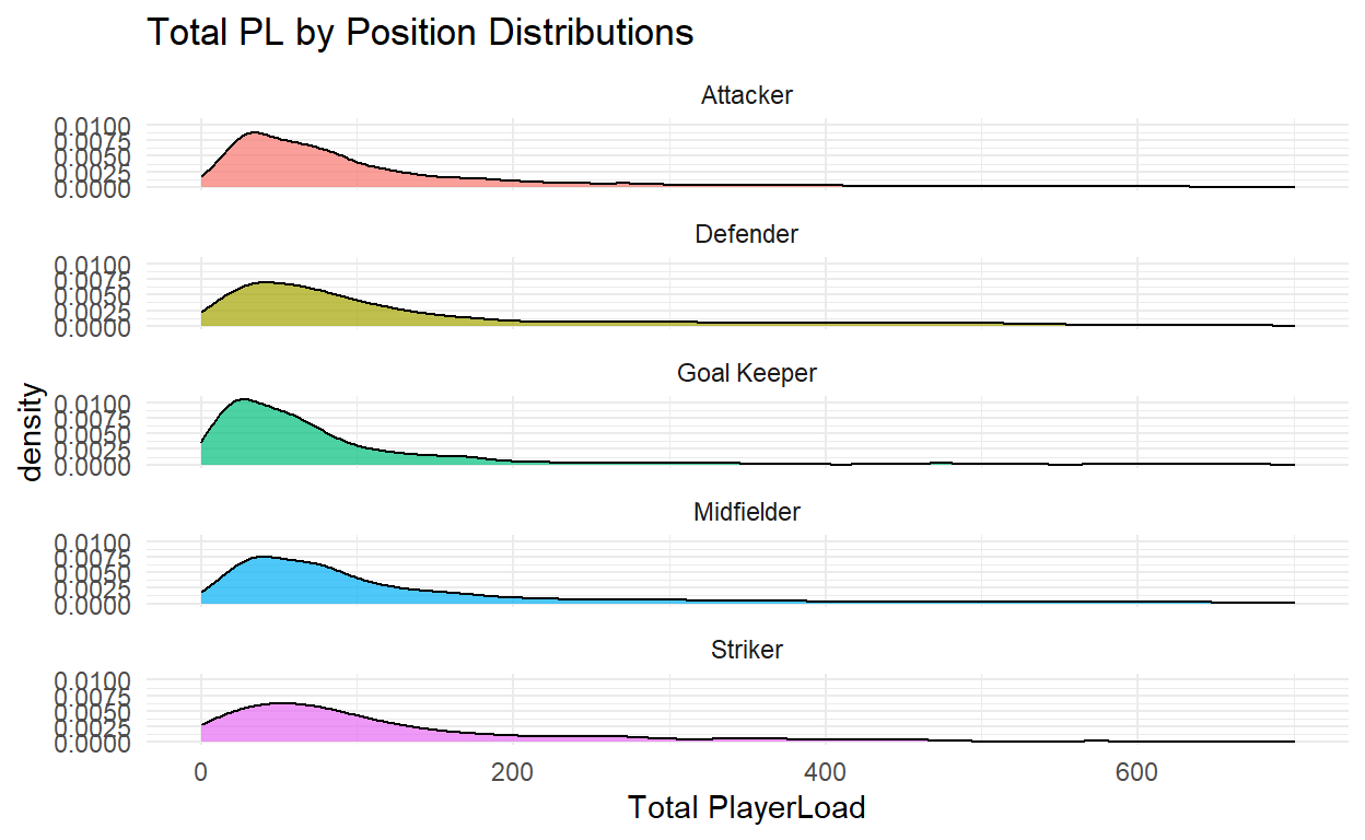
stats_df_filtered %>%
  dplyr::filter(max_vel < 20,
                date > max(date) - 100) %>%
  ggplot(aes(x = date, y = max_vel)) +
  geom_point(aes(color = position_name), alpha = 0.15) +
  geom_smooth(aes(color = position_name), se = FALSE) +
  theme_minimal() +
  theme(legend.position = "top",
        legend.title = element_blank()) +
  labs(title = "Max Velocity by Position",
       subtitle = "Most Recent 100 Days",
       x = "Date",
       y = "Max Velocity (m/s)") +
  scale_y_continuous(limits = c(0, 10))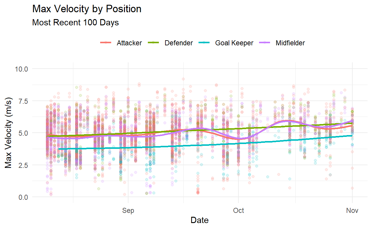
Conclusion
You have now accessed some data and can begin a more detailed analysis if you wish. For other types of data requests, proceed to another section of the Quick Start Tutorial.
Contact: datascience@catapultsports.com (email) | #ask_catapultR (Slack)